


Descriptive summary reference
This study reports the mean, median, SD, CV, quartiles, a confidence interval for the mean and distribution plots for each level, with any limit set.
Settings
Section titled “Settings”The experimental unit is the specimen. The statistics use every included row, but a limit needs at least 2 different specimen IDs. Repeated specimen IDs turn off the mean interval; see Independent results.
Analyte and Unit are required. Confidence level, Measurement scale, Display decimal places and Permit negative results are calculation settings.
Columns
Section titled “Columns”| Column | Required? | What to enter |
|---|---|---|
| Specimen / material ID | Repeated specimens | A coded ID, for example 00001, with no patient identifiers. A result without one is numbered S1, S2… when you save |
| Result | Yes | The measured value. Negative values need Permit negative results |
| Level | No | A group name, for example 1 or High. A file without a Level column puts every row in level 1 |
In Import a file, the column uses are Specimen or material ID, Result and Level or group; a file without an ID column gets generated IDs. An imported file can also hold Day, Run and Replicate; the grid does not show them.
The calculation stops on a marked row (see Validation messages), a blank analyte or unit, or when every row is excluded.
Acceptance limits
Section titled “Acceptance limits”- The unrounded estimate is compared with the limit, and a result exactly on the limit meets it.
- A CV limit is in
%; the others are in the study unit, and a limit in another unit is Undecided. - A level with fewer than 2 different specimen IDs, or an estimate that can't be calculated, is Undecided.
- On an interval scale, CV and percentage limits are not calculated; an absolute limit in the study unit is. An SD limit requiring both a study-unit and percentage allowance is Not met when its study-unit requirement fails and Undecided otherwise.
- A limit that is Not met makes the whole study Criteria not met.
See Set acceptance limits for the choices and About acceptance decisions.
Results and plots
Section titled “Results and plots”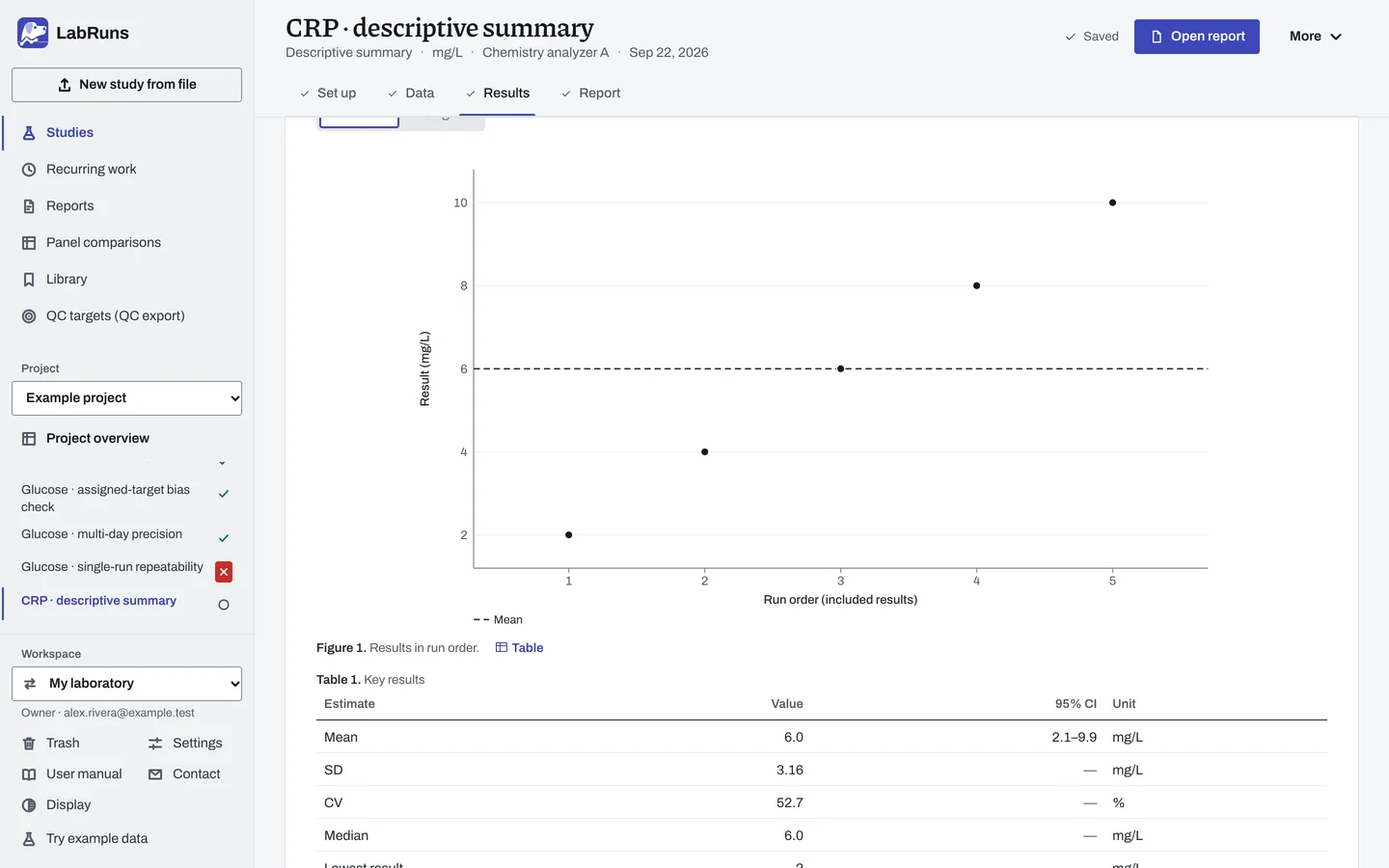
- Results: the mean with its confidence interval, SD, CV, median and lowest and highest results, arranged as described in Reading results. With more than one level, Results by level gives one row per level and Acceptance criteria lists each limit.
- With more than one level, Additional estimates gives the median and the lowest–highest range.
- Results plot: results in entry order with the mean as a dashed line. Histogram switches the plot to bars; Run order switches back. Selecting a point finds its row.
- Supporting diagnostics: a Q–Q plot and a box plot with every point.
- Additional statistics: every statistic, including variance, quartiles, the mean CI and geometric statistics for positive ratio-scale results. The Calculation selector opens earlier calculations.
Example
Section titled “Example”descriptive.csv holds five results (2, 4, 6, 8, 10) from specimen IDs 00001 to 00005, all in level 1.
Settings:
- analyte
Example analyte, unitmmol/L, 3 display decimals - 95% confidence
- limits CV at most
60% and Mean from5to7mmol/L
| Estimate | Displayed value |
|---|---|
| Mean | 6.000 mmol/L |
| Median | 6.000 mmol/L |
| Sample SD | 3.162 mmol/L |
| CV | 52.70% |
| Minimum / Maximum | 2.000 / 10.000 mmol/L |
| 25th / 75th percentile | 4.000 / 8.000 mmol/L |
| 95% CI for mean | 2.074–9.926 mmol/L |
| Acceptance limit | Observed | Limit | Outcome |
|---|---|---|---|
| CV | 52.70% | ≤ 60% | Met |
| Mean | 6.000 mmol/L | 5–7 mmol/L | Met |
The study status is Criteria met. Without limits, the report's outcome reads Descriptive results. The box plot shows quartiles 4, 6 and 8 with whiskers at 2 and 10.
Calculations and sources
Section titled “Calculations and sources”When you calculate CRP · descriptive summary in the example project, LabRuns records these methods:
- Arithmetic mean, and sample SD with an n − 1 denominator.
- Quantiles use linear interpolation (Hyndman–Fan type 7). The histogram has ⌈√n⌉ equal-width bins, at most 40.
- Two-sided 95% Student t CI for the mean.
- Results are grouped by concentration level. Every included result is used.
- Criteria evaluate the unrounded estimates.
- SD allowances using a percentage require a ratio scale. With both limits required on an interval scale, a failed study-unit requirement fails the criterion; otherwise it is undecided.
- Distribution diagnostics: ordered values plotted against standard-normal quantiles at Blom positions pᵢ = (i − 3/8)/(n + 1/4).
- Box: type-7 quartiles, IQR = Q3 − Q1. Whiskers end at the most extreme values within Q1 − 1.5 IQR and Q3 + 1.5 IQR. Values beyond the whiskers stay in the analysis.
- Q–Q and box plots need at least 3 values that are not all identical. The strip plot shows every included value.
- For positive ratio-scale data, geometric mean = exp(mean(ln x)); geometric SD = exp(sample SD(ln x)), using n−1. The two-log-SD interval is exp(mean(ln x) ± 2·SD(ln x)); it is a descriptive spread interval. Multiplicative spread = 100·(geometric SD−1)%, a multiplicative measure that differs from the coefficient of variation.
For each level:
| Estimate | How it is calculated |
|---|---|
| Variance | SD² |
| CV | 100 × SD / mean. Needs a ratio scale, at least 2 results, a positive mean and no negative results |
| Minimum, Maximum | Smallest and largest included result |
| Mean CI | mean ± t(1 − α/2, n − 1) × SD / √n |
Sources: NIST/SEMATECH e-Handbook §1.3.5.6 and §1.3.5.2, Blom (1958), and Hyndman and Fan (1996). See Study reference.