


Reference interval establishment reference
Reference interval establishment calculates new reference limits from your own healthy subjects: a two-sided reference interval or a one-sided lower or upper limit, for each partition. Each limit has a two-sided confidence interval showing how precisely it is estimated.
Settings
Section titled “Settings”| Setting | Where | Default | Meaning |
|---|---|---|---|
| Reference limits | New study and Set up | Two-sided | Two-sided interval (lower and upper limits), one-sided lower reference limit or one-sided upper reference limit |
| Target population coverage (0–1) | Set up | 0.95 |
The share of the healthy population inside the interval. A two-sided 95 % interval leaves 2.5 % in each tail. A one-sided upper 95 % limit leaves 5 % above it. See population coverage |
| Estimator | Set up | Automatic for each partition | See Estimators and transformations |
| Data transformation | Set up, shown | Set by the estimator | See Estimators and transformations |
| Confidence level | Calculation settings | 90 % | 90 %, 95 % or 99 %, for the interval around each limit. A one-sided limit still gets a two-sided confidence interval. See confidence level |
Design
Section titled “Design”- Independent healthy subjects who meet your eligibility rules. Each subject counts once. Repeat draws are averaged and flagged.
- Optionally partitions, for example
femaleandmale, each with its own limits. Without a partition column, all subjects are in partition1. - The counts to collect are in the collection plan under Run this study.
Estimators and transformations
Section titled “Estimators and transformations”- Automatic for each partition (default): uses nonparametric limits at 120 or more eligible subjects. With 20 to 119, it checks the original values with Shapiro–Wilk at a 0.05 threshold, then the log10 values when every measurement is positive. A supported Gaussian model selects parametric limits; a supported log-Gaussian model selects log-normal limits within its supported coverage and confidence settings. Otherwise it uses nonparametric limits where estimable. With fewer than 20 subjects the diagnostic is recorded and no distribution model is selected, so the nonparametric minimum for the selected coverage and sidedness applies. At the default 95% two-sided coverage, that minimum is 39 and no limits are printed. The saved result identifies the chosen method and diagnostic, and the report prints them beside the limits on page 1.
- Nonparametric percentiles: limits at rank p(n + 1) with exact confidence intervals.
- Parametric (normal theory): assumes a normal distribution.
- Log-normal (approximate CIs): assumes the log10 values are normal. It needs two-sided limits, coverage 0.95, confidence 90 %, 95 % or 99 %, and positive values. Limit CIs are approximate.
Data transformation is selected separately for each partition in automatic mode. For a manual estimator it is shown beside the estimator and set by it: None, or Base-10 logarithm for log-normal. Results are reported in the study unit.
Why the method matters is in Choosing an estimator.
Minimum subject counts
Section titled “Minimum subject counts”| Setting | Subjects needed | With fewer |
|---|---|---|
| Nonparametric two-sided limits at 95% coverage | 39 | No limits |
| Confidence interval on a nonparametric two-sided 95% limit, 90% confidence | 119 | Limits, but no CI |
| Confidence interval on a nonparametric two-sided 95% limit, 95% confidence | 146 | Limits, but no CI |
| Nonparametric one-sided limit (lower or upper) at 95% coverage and its CI, 90% confidence | 59 | No limit and no CI |
| The same at 95% confidence | 72 | No limit and no CI |
| Parametric or log-normal limits, chosen by hand | 2 | No limits |
| A distribution model under Automatic | 20 | Nonparametric minima apply |
Other coverage and confidence settings need other counts. The result gives the number.
Columns
Section titled “Columns”| Column use | Grid column | Required | What to enter |
|---|---|---|---|
| Specimen or material ID | Subject ID | Yes | Coded ID of the reference subject, one per person (no names). Repeat draws share the subject's ID |
| Result | Result | Yes | The measured value. The analysis needs exact values |
| Level or group | Partition | No | The reference group, for example female |
| Replicate | Replicate | No | Draw number, for your records |
Day and Run can be imported but aren't shown in the grid. See Importing and mapping and Column reference.
The calculation stops until these are fixed:
- a missing analyte or unit;
- a subject entered in two partitions;
- a cohort with no eligible subjects;
- rows marked with errors.
Too few subjects does not stop the calculation. The result gives the count and explains why the limits weren't calculated.
Acceptance limits
Section titled “Acceptance limits”The dialog is in Set acceptance limits. For this study:
- A limit applies to the Lower reference limit or the Upper reference limit, with a Lower limit, an Upper limit or both.
- The limit is compared with the reference limit itself, in the study unit. The CI width doesn't enter.
- A reference limit that wasn't calculated gives Undecided.
See About acceptance decisions.
Results and plots
Section titled “Results and plots”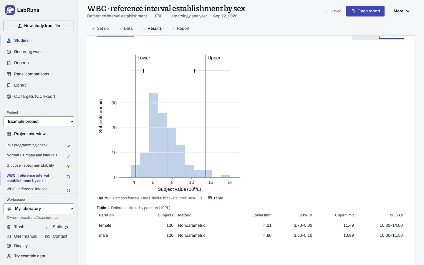
The summary and overview show every partition. With several, Partition details chooses the partition whose supporting details are shown.
- Reference limits by partition gives each partition's subjects, the method with its Shapiro–Wilk p value under automatic selection, and each limit with its two-sided CI.
- Subject values and limit CIs by partition adds the mean, SD, observed range and the CI ranks. Automatic selection also shows the method and normality diagnostic used for each partition. The reason for any "Not estimated" is below the table.
- Estimator details · partition under Detailed statistics holds the estimator, assumptions, sample-size and tail checks, exclusions and CI ranks.
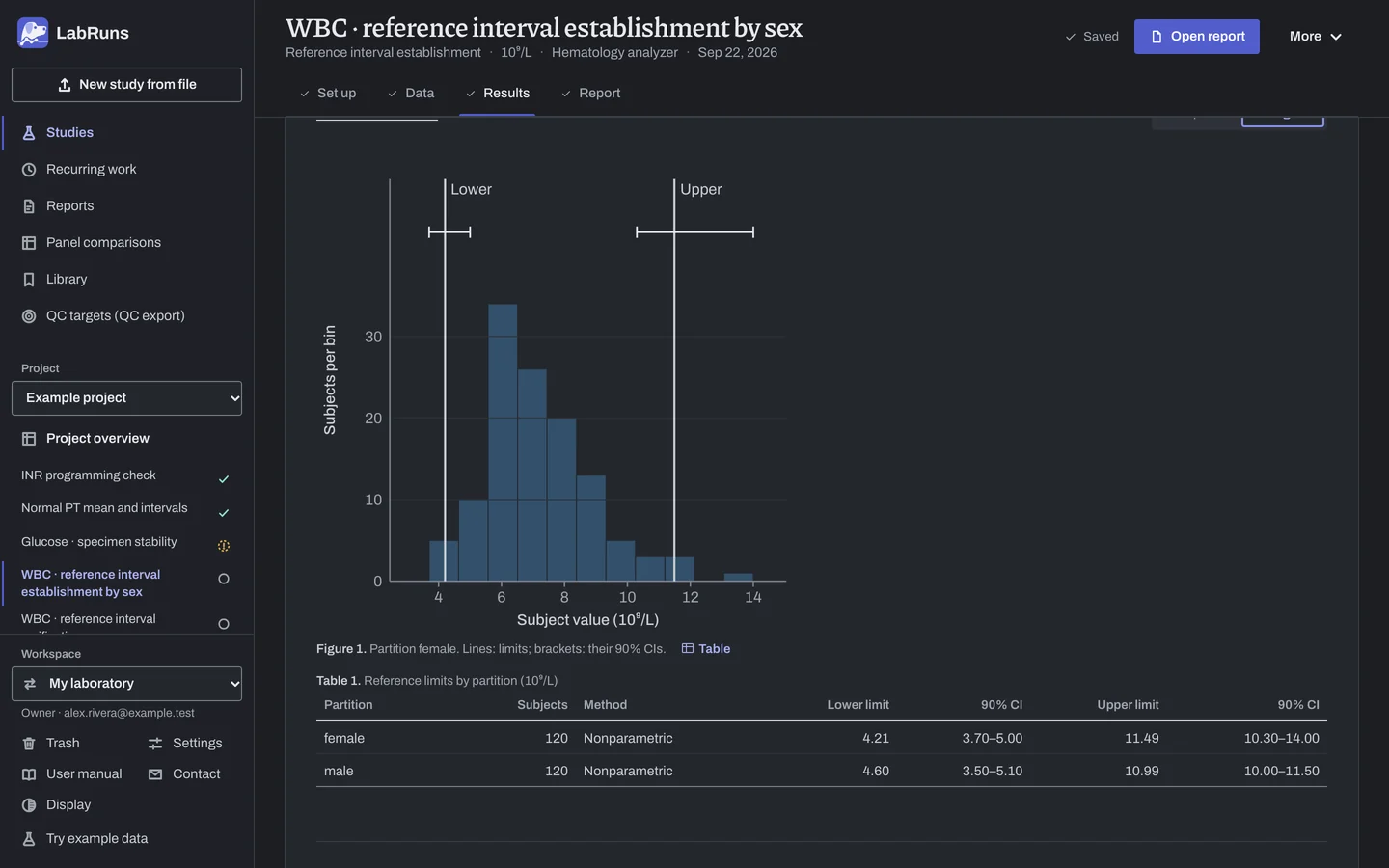
- The plot shows a histogram of each partition with lines at the limits and brackets for their CIs. It switches between Histogram and Raw points.
- Review values outside 1.5·IQR whiskers lists values beyond the Tukey fences, with View row links. Flagged values stay in the result.
- Including excluded rows (for information only) appears when a partition has excluded rows. It shows what the exclusions changed.
Distribution diagnostics
Section titled “Distribution diagnostics”Distribution diagnostics · partition needs at least 3 subjects whose values are not all the same:
- Normal Q–Q: a straight line suggests a roughly normal shape, a curve suggests skew, and isolated end points are tail values.
- Box and raw-point strip: the box runs from Q1 to Q3 with the median, whiskers reach the most extreme values within 1.5 × IQR, and the strip shows every subject.
Example
Section titled “Example”reference_establish_120.csv: 240 example white blood cell counts (10^9/L), 120 subjects each in female and male, one draw each.
Setup: two-sided, coverage 0.95, Nonparametric percentiles, 90 % confidence. One acceptance limit: Upper reference limit at most 12.5 10^9/L.
| Partition | Subjects | Lower limit (90 % CI) | Upper limit (90 % CI) | Upper reference limit (≤ 12.5) |
|---|---|---|---|---|
| female | 120 | 4.21 (3.70–5.00) | 11.49 (10.30–14.00) | Met (11.49) |
| male | 120 | 4.60 (3.50–5.10) | 10.99 (10.00–11.50) | Met (10.99) |
The study status is Criteria met.
- CI on estimated limits: the lower limit's CI uses order statistics 1 and 7, the upper's 114 and 120. Because ranks are whole numbers, achieved coverage is 92 % against the nominal 90 %.
- The female upper CI, 10.3 to 14, runs to the largest value.
- Tail estimates: 6 of 120 female values fall outside the limits, against about 6 expected. Male: 5 of 120.
- The review list flagged 3 female values (
F08011.5,F00111.8,F11214; upper fence 11.250) and 1 male value (M03311.5; upper fence 11.263). They stay in the result.
Excluding a flagged subject
Section titled “Excluding a flagged subject”In a second study, row F112 (14.0) was excluded with a reason. Female result:
| Measure | Result · exclusions applied | Including excluded · descriptive |
|---|---|---|
| Independent subjects | 119 | 120 |
| Draws | 119 | 120 |
| Lower reference limit (10⁹/L) | 4.20 | 4.21 |
| Upper reference limit (10⁹/L) | 11.20 | 11.49 |
The upper 90 % CI became 10.00 to 11.80.
A one-sided upper limit
Section titled “A one-sided upper limit”On the 120-subject file, a one-sided upper limit at 90 % confidence gave female 10.40, CI 9.60–11.80, and male 10.48, CI 9.70–11.00. Each had 6 of 120 values above.
A cohort that is too small
Section titled “A cohort that is too small”reference_establish.csv has 41 rows: 20 female subjects (F019 has two draws, averaged) and 20 male. With the nonparametric estimator, every limit and CI shows —, and the note gives the reason: two-sided limits need 39 subjects. Parametric (normal theory) gives, for example, female 3.232 to 10.763 10^9/L, with 90 % CIs of 1.940–4.523 on the lower limit and 9.472–12.055 on the upper.
Calculations and sources
Section titled “Calculations and sources”When you calculate WBC · reference interval establishment by sex in the example project, LabRuns records these methods:
- Automatic reference method choice is per partition: at least 120 eligible subjects uses nonparametric limits. With 20 to 119 subjects, Shapiro–Wilk p ≥ 0.05 supports normal-theory limits; otherwise positive values with Shapiro–Wilk p ≥ 0.05 after log10 transformation support log-normal limits, within their supported settings. If neither model is supported, or there are fewer than 20 subjects, nonparametric calculation minima apply. A normality test does not establish normality.
- Nonparametric limits are the values at rank p(n+1) (Hyndman–Fan type 6, linear interpolation) for p = (1−coverage)/2 and 1−(1−coverage)/2. At 95% coverage they need at least 39 subjects. Each limit has an exact binomial order-statistic CI.
- Parametric limits are mean ± z·s and assume a Gaussian reference distribution. Limit CIs use SE = s·√(1/n + z²/(2(n−1))) with a t(n−1) multiplier.
- Repeat draws from one subject are averaged into one value. The distribution histogram uses ceil(√n) equal-width bins, at most 40.
- At least 120 eligible subjects per partition are recommended. Each partition is analyzed on its own.
- Distribution diagnostics: ordered values plotted against standard-normal quantiles at Blom positions pᵢ = (i − 3/8)/(n + 1/4).
- Box: type-7 quartiles, IQR = Q3 − Q1. Whiskers end at the most extreme values within Q1 − 1.5 IQR and Q3 + 1.5 IQR. Values beyond the whiskers stay in the analysis.
- Q–Q and box plots need at least 3 values that are not all identical. The strip plot shows every included value.
- Reference review: Tukey 1.5·IQR screening using the type-7 quartiles. Values outside Q1 − 1.5·IQR or Q3 + 1.5·IQR are flagged for review. Values equal to a fence are not flagged.
- Nonparametric one-sided limits use
p = coverage(upper) orp = 1 − coverage(lower). Two-sided limits needn ≥ 1/p − 1. - Limit CI: ranks
randswith each tail at mostα/2, achieved coverageP(r ≤ B ≤ s − 1),B ~ Binomial(n, p). If a rank falls outside1…n, there is no CI. Horowitz 2008 gives ranks 1–7 and 114–120 at n = 120, 90 %. - Parametric limits use
z = Φ⁻¹((1 + coverage)/2)two-sided orΦ⁻¹(coverage)one-sided (Bland). Identical values put both limits at that value and withhold both limit confidence intervals. - Log-normal limits:
m ± z·son the log10 scale withz = Φ⁻¹(0.975), back-transformed as10^x. Each limit CI has log-scale half-widthΦ⁻¹((1 + confidence)/2) · s · √((1 + z²/2)/n). Achieved coverage is unknown. Values at or below zero, or identical log values, stop the analysis.
See Study reference.
Evidence references: CAP COM.40605, COM.40615 (9 December 2025). In a binder, the CAP evidence index lists the report sections behind each requirement and the laboratory records that go with them.