


Method comparison reference
A method comparison measures the same patient specimens on a test method and a comparative method. It reports each specimen's difference against its allowable difference, four regression fits, the mean difference with 95% limits of agreement, and bias at medical decision levels. The test method is the y-axis and the comparative method the x-axis. Every difference is test minus comparative: a positive bias means the test method reads higher.
Settings
Section titled “Settings”| Setting | Meaning |
|---|---|
| Comparative method or instrument, Test method or instrument | Asked in New study. The comparative method is plotted on the x-axis |
| Medical decision levels | Up to 10 concentrations in the study unit, separated by semicolons. Bias is estimated at each level |
| Primary regression | Passing-Bablok · robust (default), Deming · constant SD, Weighted Deming · constant CV or Ordinary least squares. See The four regressions |
| How λ is supported | See How the Deming ratio is supported |
| Plot relative differences (%) | Under Calculation settings. The difference plot shows 100 × (test − comparative) ÷ |comparative result|, skipping exact zeros |
| Measurement scale | Under Calculation settings. Percentage statistics and weighted Deming need a ratio scale with a meaningful zero |
| Claimed lower reportable limit, Claimed upper reportable limit | Under Reportable-range coverage (optional). With both, the saved result shows the percentage of that interval spanned by matched specimen means on the comparative method. It describes the tested span. Acceptance and reportable-range verification are separate |
Specimens and counts
Section titled “Specimens and counts”The experimental unit is the specimen (definition). Rows with the same specimen ID are averaged into one pair. Replicates can support the Deming ratio.
| Count | What happens |
|---|---|
| Fewer than 2 specimens with included pairs | No calculation. |
| Fewer than 3 specimens | No slope or intercept intervals. |
| Fewer than 5 specimens | No Passing-Bablok slope or intercept intervals. |
| Fewer than 5 specimens | The specimen limit is Undecided. |
The four regressions and what each needs
Section titled “The four regressions and what each needs”All four fits use the specimen means. The limits, decision-level table, residual plot and band use the Primary regression. A fit that can't run shows why in the table. Choosing a regression explains when each suits.
| Primary regression | Needs |
|---|---|
| Passing-Bablok · robust (default) | A positive, roughly linear relationship |
| Deming · constant SD | λ |
| Weighted Deming · constant CV | λ, and all values above zero |
| Ordinary least squares | Nothing extra |
How the Deming ratio is supported
Section titled “How the Deming ratio is supported”For a Deming or weighted Deming fit, λ is the test method's error variance divided by the comparative method's. λ = 1 means both methods are equally imprecise.
| How λ is supported | What happens |
|---|---|
| Computed from replicate pairs in this study | Needs at least 2 specimens with at least 2 replicate pairs each, or neither Deming fit runs. |
| Taken from linked precision studies | Uses multi-day precision or repeatability studies of the same analyte and unit in this project. |
| Stated assumption | Uses the Assumed error-variance ratio λ entered, or 1 when it is blank. |
Until a basis is chosen, the study uses Computed from replicate pairs in this study when every specimen has at least 2 replicate pairs, and Stated assumption with λ = 1 otherwise. The saved result names the basis it used.
Linked precision results
Section titled “Linked precision results”The Test method (y) and Comparative method (x) pickers list precision results for this analyte and unit in this project, one entry per level. A linked level needs an SD above 0.
A link goes stale when the linked study gets new data or a new calculation. The link keeps the result that was chosen and never moves to the newer one by itself. Results, new report copies, CSV downloads and the project report show Results out of date. A new calculation still uses that earlier result and warns that the linked study changed. With a Deming primary fit, the slope, intercept and decision-level bias limits are then Undecided and no band is drawn; mean-bias and specimen limits are decided as usual. A calculation with a stale link can't be signed off, and a calculation saved while the link was current can't be returned again once it goes stale. Linking precision studies gives the steps.
Columns
Section titled “Columns”| Column use | Grid column | Required? | What to enter |
|---|---|---|---|
| Specimen or material ID | Specimen ID | Yes | Coded ID, repeated on every replicate row of that specimen |
| Comparative method result | Comparative method (x) | Yes | Comparative result, in the study unit |
| Test method result | Test method (y) | Yes | Test result for the same specimen, on the same row |
| Level or group | Specimen group (level) | No | A group label such as outpatient, the same on every replicate row. It appears in each plot point's label. With two or more groups, each group of at least 5 specimens gets its own marker and colour in the plots, named in the legend |
| Replicate | Replicate | No | Replicate label |
The template and exported files call the two results comparator and candidate. Import recognizes common headers such as comparator, reference or x, and candidate, test or y; see Headings the app recognizes. The optional Excluded and Exclusion reason columns are in Fields every study type offers.
The primary regression can't run with weighted Deming and a zero value, or with a Deming ratio that is not a positive number.
Acceptance limits
Section titled “Acceptance limits”The specimen rule decides agreement: at least 95% of specimens, rounded up, must be within their limits. With 5–19 specimens all must be, with 20 specimens 19, with 25 specimens 24. A percentage limit needs a comparative result above zero on a ratio scale. A specimen that can't be evaluated leaves the limit Undecided unless enough specimens already fail: with 20 specimens, 1 failure and 1 not evaluated is Undecided, 2 failures and 1 not evaluated is Not met. See About acceptance decisions.
Without a specimen rule, a built-in Specimen agreement check stays Undecided and the study can't reach Criteria met. The other limits check point estimates from the primary fit.
- Slope limits are in
ratio, Mean relative bias (%) limits in%, and every other limit in the study unit. A limit in another unit is Undecided; the report keeps its entered unit and leaves that criterion's observed value blank. Specimen rules, including percentage rules, use the study unit. - A Mean relative bias (%) limit divides each difference by the comparative result, skipping exact zeros. It is decided whether or not Plot relative differences (%) is ticked.
- A decision-level limit sets its own Medical decision level, separate from the list on Set up. On an interval scale, a decision-level bias limit requiring both study-unit and percentage allowances is Not met when its study-unit requirement fails and Undecided otherwise. The acceptance table keeps both requirements visible.
- A decision level outside the range of comparative specimen means is extrapolated, and any limit at that level is Undecided.
- A concentration-dependent specimen rule picks its segment by each specimen's comparative result, and decision-level bias by the decision level. A specimen or level in a gap is not evaluated. See Concentration-dependent limits.
Results and plots
Section titled “Results and plots”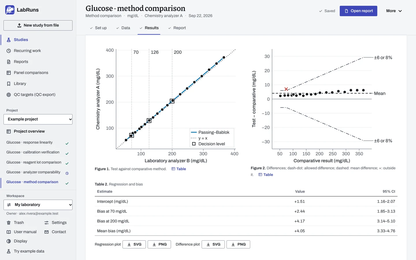
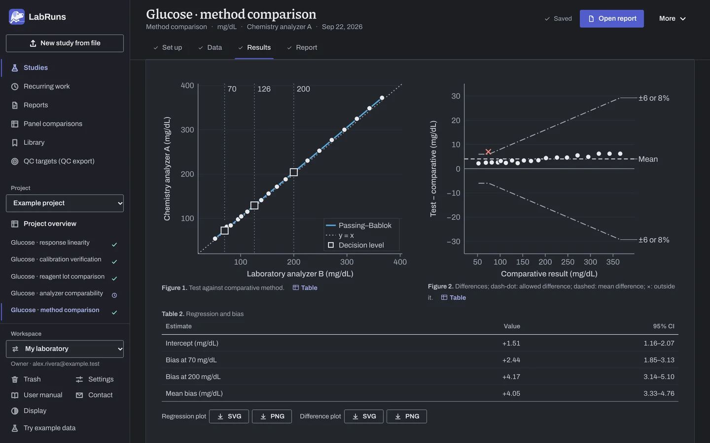
Regression plot. One point per specimen, mean test against mean comparative. The dashed line is the primary fit across the observed range. The dotted line is y = x, and points above it read higher on the test method. Selecting a point jumps to its row. The strip under it gives the specimen count and the range covered.
Slope and intercept by regression method lists all four fits, each with its interval under it (for example 95% CI 1.012–1.016), marks the primary one and gives Pearson r under it. With a Deming primary fit, Ranges and fit details gives the λ used and its basis. Pearson r prints as > 0.9999 when it rounds to 1. The slope has no unit. Bias at medical decision levels gives each level's estimated bias, its interval and whether the level is inside the studied range.
The decision table, under the verdict, shows Outcome, Criterion, Observed and Acceptance limit for each criterion. Below the figures, Specimen decisions expands to each specimen's comparative result, difference, allowed difference and outcome. The report gives the same table; both results are in its data listing.
Difference plot and summary. Test minus comparative for each specimen, against the comparative result, with the mean bias and 95% limits of agreement. Labels in the right margin give their values in the plot's unit, for example Mean +4.05, LoA +1.04 and LoA +7.05. With Plot relative differences (%) ticked, the plot shows relative differences. Bias intervals and independent results explains how the interval of the mean bias and the limits of agreement differ.
Allowable-difference marks. Short marks at each specimen show mean-bias, mean-relative-bias and concentration-dependent decision-level limits. In the example they show the 200 mg/dL limit (±4 mg/dL below 100 mg/dL, ±4 % from 100 mg/dL up) and the ±5 mg/dL mean-bias limit. The specimen rule's limits are in Specimen decisions.
Imprecision caution. With replicate pairs, or precision studies linked for λ, the two methods' pooled repeatability SD gives the SD of a matched difference from imprecision alone (√(2/k) times the repeatability SD for k replicates per specimen). When the specimen allowance at the mean comparative result is below 1.96 times that SD, the results carry a caution with the share of specimens imprecision alone would put outside the allowance. The caution changes no decision.
Residual diagnostic. Test result minus the primary fitted value, against the comparative result. A pointwise band at the study's confidence level, shaded on the regression plot, shows how well the line is known. It appears for an OLS fit, or a Deming or weighted Deming fit with a current λ basis, with at least 3 specimens.
The report. Page 1 puts the regression plot beside each specimen's difference, drawn against its allowed difference (dashed; a specimen outside it is a cross). One table under them gives the primary slope and intercept, the bias at each decision level and the mean bias, each with its CI, limit and result, and how many specimens are within their allowed difference. The data listing starts on page 2. Specimen decisions, the difference plot with the 95% limits of agreement (relative differences when Plot relative differences (%) is ticked) and the fit details follow it. The other regressions and the residual plot are added by Include technical details.
Example
Section titled “Example”comparison.csv holds 20 example glucose specimens, one pair each, comparative results 52.1 to 365.9 mg/dL.
| Setting | Value |
|---|---|
| Analyte, unit | Glucose, mg/dL |
| Comparative method (x) / Test method (y) | Laboratory analyzer B / Chemistry analyzer A |
| Confidence level | 95% |
| Primary regression | Passing-Bablok |
| How λ is supported | Stated assumption (λ = 1, preset because the file has no replicates) |
| Plot relative differences (%) | Ticked |
| Medical decision levels | 70; 126; 200; 400 |
The specimen rule allows 6 mg/dL or 8% of the comparative result, whichever is greater. It becomes the segments 0,75,absolute,6 and 75,,relative,8. The 200 mg/dL limit uses the segments 0,100,absolute,4 and 100,,relative,4. All limits are inclusive.
Results as the screen shows them:
| Estimate | Value | 95% confidence interval |
|---|---|---|
| Mean bias, test minus comparative | +4.05 mg/dL | 3.33–4.76 |
| SD of differences | 1.53 mg/dL | |
| 95% limits of agreement | +1.04 to +7.05 mg/dL | lower −0.20 to 2.29; upper 5.80–8.29 |
| Mean relative bias (|comparative result| denominator) | +2.71% | 1.89–3.52 |
| Regression | Slope (interval) | Intercept, mg/dL (interval) |
|---|---|---|
| Ordinary least squares (y on x) | 1.011 (1.006–1.017) | +2.03 (0.92–3.15) |
| Deming | 1.011 (1.005–1.017) | +2.02 (0.46–3.58) |
| Weighted Deming (constant CV) | 1.009 (0.998–1.020) | +2.39 (0.19–4.60) |
| Passing-Bablok · primary | 1.013 (1.010–1.015) | +1.51 (1.16–2.07) |
Pearson r is > 0.9999.
| Medical decision level (mg/dL) | Estimated bias (mg/dL) | Interval | Inside studied range |
|---|---|---|---|
| 70 | +2.44 | 1.85–3.13 | Yes |
| 126 | +3.19 | 2.41–3.98 | Yes |
| 200 | +4.17 | 3.14–5.10 | Yes |
| 400 | +6.83 | 5.11–8.14 | No (extrapolated, can't pass) |
| Limit name | Limit | Observed | Outcome |
|---|---|---|---|
| Specimen differences | Each specimen within ±6 mg/dL or 8%, whichever is greater | 19/20 (95.00%) | Met |
| Slope | 0.950–1.050 | 1.013 | Met |
| Intercept | ±5 mg/dL | +1.51 mg/dL | Met |
| Bias at 126 mg/dL | ±6 at 126 mg/dL | +3.19 mg/dL | Met |
| Bias at 200 mg/dL | ±8 at 200 mg/dL (concentration-dependent: ±4 mg/dL below 100, ±4% from 100) | +4.17 mg/dL | Met |
| Mean bias | ±5 mg/dL | +4.05 mg/dL | Met |
The study meets its criteria. A note flags the extrapolated 400 mg/dL level. Specimen 00003 (74.0 mg/dL comparative, 81.0 test) is the one specimen outside its allowance. The test method reads about 4 mg/dL higher, and the bias grows with concentration. The example project's Glucose · method comparison uses decision levels 70, 126 and 200 mg/dL, leaves Plot relative differences (%) unticked and sets three of these limits (specimen differences, slope and bias at 126 mg/dL); all are Met.
Deming example. The same data with a Deming primary fit, decision level 126 mg/dL, the specimen rule above and three more limits: Slope 0.95 to 1.05, Bias at 126 mg/dL within ±6 mg/dL (estimate +3.43, interval 2.59–4.26) and Mean bias within ±5 mg/dL. With the preset Stated assumption (λ = 1), every limit is Met and the study status is Criteria met.
Replicate-derived λ. Three specimens with three replicate pairs each:
specimen_id,comparator_result,candidate_result
A,10,10
A,11,12
A,12,14
B,19,21
B,21,23
B,20,25
C,30,33
C,32,34
C,34,35
Every specimen has replicate pairs, so Computed from replicate pairs in this study is preset. It gives λ = 1.5 from 3 specimens, with 6 df per method. The within-specimen SDs are 1.7 mg/dL for the test method and 1.4 mg/dL for the comparative method. The 20-specimen file has no replicates, so this basis stops a Deming calculation on it.
Calculations and sources
Section titled “Calculations and sources”When you calculate Glucose · method comparison in the example project, LabRuns records these methods:
- Residuals are the test result minus the result fitted by the primary regression line.
- The fitted-response confidence band is pointwise. OLS uses Student t(n−2) with the residual SD and leverage. Deming fits use Linnet’s jackknife t(n−2) intervals. Weighted Deming iteration uses a shared concentration scale and a convergence tolerance of 1e-10.
- Comparative results are x and test results are y. Replicate pairs are averaged to one mean pair per specimen.
- Ordinary least squares fits y on x. It assumes the comparative method has negligible error and the test errors have constant variance.
- Deming regression uses λ = Var(test error)/Var(comparative error) = 1.000, with constant error variance on both axes. λ is an assumed error-variance ratio. Weighted Deming assumes spread proportional to concentration and needs results above zero. Both use jackknife t(n−2) intervals.
- Passing-Bablok is the shifted median of pairwise slopes, with rank-based CIs. It assumes a positive linear relationship and similar error distributions on both axes.
- The 95% limits of agreement are mean bias ± 1.96 SD. Mean bias has a 95% Student t CI, and the limits have CIs from SE = √(3s²/n). The CI is for the mean bias. The limits of agreement are for individual differences.
- Slope, intercept and bias at each medical decision level come from the primary fit. Bias outside the studied range is inconclusive. Criteria evaluate the unrounded estimates.
- Pearson r, from the least-squares fit, describes linear association and grows with the studied range.
- A specimen allowance below 1.96 × the SD of a matched difference from imprecision alone (the pooled repeatability SD of the two methods, from replicate pairs or linked precision studies, times √(2/k) for k replicates per specimen) is cautioned with the share of specimens imprecision alone would put outside it. The caution changes no decision.
- Reportable-range coverage is the width of the overlap between the observed reference-axis range and the claimed reportable range, divided by the claimed range width, times 100. It describes the tested span; accuracy and verification of the reportable range are separate questions. Replicate results are averaged by specimen before determining the observed range.
- Specimen agreement: d = test − comparative for each specimen mean pair. The allowance at comparative result X is A, or P × X / 100, or with both limits the larger, max(A, P × X / 100) (Pass when within either (the larger allowance)) or the smaller, min(A, P × X / 100) (Pass only when within both), as chosen under With both limits. A specimen is within its limit when |d| ≤ allowance, inclusive, compared in exact decimal arithmetic on unrounded values.
- Ordinary least squares: slope and intercept intervals use Student t on n − 2 df.
- Deming: slope = (Syy − λSxx + √((Syy − λSxx)² + 4λSxy²)) / (2Sxy), with λ as defined under How the Deming ratio is supported. Weighted Deming follows Linnet (1990) with constant-CV weights. It stops after 30 iterations or at tolerance 1e-10 in the shared concentration scale.
- Passing-Bablok (1983, 1984): slopes of exactly −1 are dropped. Intercept = median of y − slope × x. There is no intercept interval when comparative values span zero.
- Replicate-derived λ = pooled within-specimen variance of y ÷ that of x, over specimens with at least 2 pairs. Linked λ = (test repeatability SD ÷ comparative repeatability SD)².
- Differences: the mean-bias CI and the CIs of the limits of agreement use t(n − 1) (Giavarina 2015).
- Bias at decision level X = intercept + (slope − 1) × X. Its interval is a Student t interval of the fitted response (OLS), a jackknife interval (Deming, weighted Deming) or the range over the corners of the slope and intercept intervals (Passing-Bablok).
- Fitted-response band (OLS): ŷ ± t × s × √(1/n + (x − x̄)²/Sxx).
- Reportable-range coverage runs from 0% to 100%. For example, comparator results from 40 to 240 mg/dL cover 71.4% of a claimed 20–300 mg/dL interval.
Sources: Study reference.
Evidence references: CAP COM.40300, COM.40350 (9 December 2025). In a binder, the CAP evidence index lists the report sections behind each requirement and the laboratory records that go with them.